R by C Contingency Table Analysis

Menu location: Analysis_Chi-square_R by C.

The r by c chi-square test in StatsDirect uses a number of methods to investigate two way contingency tables that consist of any number of independent categories forming r rows and c columns.

Tests of independence of the categories in a table are the chi-square test, the G-square (likelihood-ratio chi-square) test and the generalised Fisher exact (Fisher-Freeman-Halton) test. All three tests indicate the degree of independence between the variables that make up the table.

The generalised Fisher exact test is difficult to compute (Mehta and Patel, 1983, 1986a); it may take a long time and it may not be computed for the table that you enter. When the test has taken a second, StatsDirect shows a progress bar, which tells you which stage of its search the test is in and how much of that stage is done; the later stages take longer. If you press Cancel then the test is stopped, and the results are given without the exact P value. If the Fisher exact method cannot be computed practically then a hybrid method based upon Cochran rules is used (Mehta and Patel, 1986b); this may also fail with large tables and/or numbers. The Fisher-Freeman-Halton result is quoted with just one P value as it is implicitly two-sided.

Relating the Fisher-Freeman-Halton statistic to the Pearson Chi-square statistic:

The null hypothesis is independence between row and column categories.
Let t denote a table from the set of all tables with the same row and column margins.
Let D(t) be the measure of discrepancy.
The exact two sided P value = P [D(t) >= D(t_observed)] = sum of hypergeometric probabilities of those tables where D(t) is larger than or equal to the observed table.
In large samples the distribution of D(t) conditional on fixed row and column margins converges to the chi-square distribution with (r-1)(c-1) degrees of freedom.

The G-square statistic is less reliable than the chi-square statistic when you have small numbers. In general, you should use the chi-square statistic if the Fisher exact test is not computable. If you consult a statistician then it would be useful to provide the G-square statistic also.

These tests of independence are suitable for nominal data. If your data are ordinal then you should use the more powerful tests for trend (Armitage and Berry, 1994; Agresti, 2002, 1996).

Assumptions of the tests of independence:

the sample is random
each observation may be classified into one cell (in the table) only

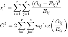
- where, for r rows and c columns of n observations, O is an observed frequency and E is an estimated expected frequency. The expected frequency for any cell is estimated as the row total times the column total then divided by the grand total (n).

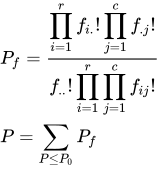
- where P is the two sided Fisher probability, P_f is the conditional probability for the observed table given fixed row and column totals (f_i. and f_.j respectively), f_.. is the total count and ! represents factorial.

Analysis of trend in r by c tables indicates how much of the general independence between scores is accounted for by linear trend. StatsDirect uses equally spaced scores (1, 2, 3 and so on) for this purpose unless you specify otherwise: if you select 'Specify trend scores' then you are asked for a score for each row and a score for each column, and the scores that are used are shown with the table. If you wish to experiment with other scoring systems then expert statistical guidance is advisable. Armitage and Berry (1994) quote an example where extent of grief of mothers suffering a perinatal death, graded I to IV, is compared with the degree of support received by these women. In this example the overall statistic is non-significant but a significant trend is demonstrated.

The sample correlation coefficient r reflects the direction and closeness of linear trend in your table. r may vary between -1 and 1 just like Pearson's product moment correlation coefficient. Total independence of the categories in your table would mean that r = 0. The test for linear trend is related to r by M²=(n-1)r² and this is numerically identical to Armitage's chi-square for linear trend (Armitage and Berry, 1994; Agresti, 1996). If you interchange the rows and columns in your table then the value of M² will be the same.

The ANOVA output applies techniques similar to analysis of variance to an r by c table. Here the equality of mean column and row scores is tested. StatsDirect uses equally spaced scores for this purpose unless you specify otherwise. See Armitage for more information (Armitage and Berry, 1994).

Pearson's and Cramér's (V) coefficients of contingency and the phi (φ, correlation) coefficient reflect the strength of the association in a contingency table (Agresti, 1996; Fleiss, 1981; Stuart and Ord, 1994):

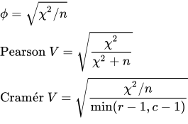
For 2 by 2 tables, Cramér's V is calculated alternatively as a signed value:

Observed values and totals are given for the table, with expected values and cell chi-square contributions if you ask for them. A row or column without any counts takes no part in the analysis: r and c above are the numbers of rows and columns that have counts.

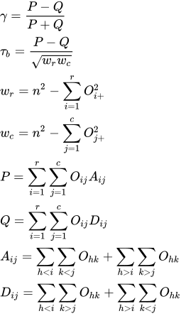
If your data categories are both ordered then you will gain more power in tests of independence by using the ordinal methods due to Goodman and Kruskal (gamma) and Kendall (tau-b). Large sample, asymptotically normal variance estimates are used; the simple form is used for independence testing (Agresti, 1984; Conover, 1999; Goodman and Kruskal, 1963, 1972). Tau-b tends to be less sensitive than gamma to the choice of response categories.

Example

From Armitage and Berry (1994, p. 408).

The following data (as above) describe the state of grief of 66 mothers who had suffered a neonatal death. The table relates this to the amount of support given to these women:

		Support
		Good	Adequate	Poor
Grief State:	I	17	9	8
	II	6	5	1
	III	3	5	4
	IV	1	2	5

To analyse these data in StatsDirect you must select r by c from the chi-square section of the analysis menu. Choose the default 95% confidence interval. Check the boxes marked "Try Fisher-Freeman-Halton exact test", "Show expected counts" and "Show cell chi-square", and clear "Show percentages". Then enter the above data as directed by the screen.

For this example:

Observed	17	9	8	34
Expected	13.909091	10.818182	9.272727
DChi²	0.686869	0.305577	0.174688
Observed	6	5	1	12
Expected	4.909091	3.818182	3.272727
DChi²	0.242424	0.365801	1.578283
Observed	3	5	4	12
Expected	4.909091	3.818182	3.272727
DChi²	0.742424	0.365801	0.161616
Observed	1	2	5	8
Expected	3.272727	2.545455	2.181818
DChi²	1.578283	0.116883	3.640152
Totals:	27	21	18	66

TOTAL number of cells = 12

Warning: 9 out of 12 cells have EXPECTATION < 5

NOMINAL INDEPENDENCE

Chi-square = 9.9588, DF = 6, P = 0.1264

G-square = 10.186039, DF = 6, P = 0.117

Fisher-Freeman-Halton exact P = 0.1426

ANOVA

Chi-square for equality of mean column scores = 5.696401

DF = 2, P = 0.0579

LINEAR TREND

Sample correlation (r) = 0.295083

Chi-square for linear trend (M²) = 5.6598

DF = 1, P = 0.0174

NOMINAL ASSOCIATION

Phi = 0.388447

Pearson's contingency = 0.362088

Cramér's V = 0.274673

ORDINAL

Goodman-Kruskal gamma = 0.349223

Approximate test of gamma = 0: SE = 0.15333, P = 0.0228, 95% CI = 0.048701 to 0.649744

Approximate test of independence: SE = 0.163609, P = 0.0328, 95% CI = 0.028554 to 0.669891

Kendall tau-b = 0.236078

Approximate test of tau-b = 0: SE = 0.108929, P = 0.0302, 95% CI = 0.02258 to 0.449575

Approximate test of independence: SE = 0.110601, P = 0.0328, 95% CI = 0.019303 to 0.452852

Here we see that although the overall test was not significant we did show a statistically significant trend in mean scores. This suggests that supporting these mothers did help lessen their burden of grief.

R code

This R code reproduces the example above. It needs no packages and was checked with R 4.6.1. Paste it into R, or save it as a script and run it.

# R by c contingency table: the StatsDirect help example (Armitage and Berry 1994,
# grief of 66 mothers after a neonatal death by the support they received) in R
counts <- matrix(c(17, 9, 8,
                   6, 5, 1,
                   3, 5, 4,
                   1, 2, 5), 4, 3, byrow = TRUE,
                 dimnames = list(Grief = c("I", "II", "III", "IV"),
                                 Support = c("Good", "Adequate", "Poor")))
print(addmargins(counts))
n <- sum(counts)
six <- function(x) formatC(x, digits = 6, format = "f", drop0trailing = TRUE)
pv <- function(p) {
  if (p < 0.0001) "P < 0.0001" else
    paste("P =", formatC(p, digits = 4, format = "f", drop0trailing = TRUE))
}

# Nominal independence: Pearson's chi-square without Yates' correction (R warns
# that the expected counts are small, as the report does), the expected counts
# and each cell's share of the chi-square, the likelihood ratio G-square and the
# Fisher-Freeman-Halton exact test, which fisher.test gives for a table larger
# than 2 by 2
chi <- suppressWarnings(chisq.test(counts, correct = FALSE))
cat("Expected\n")
print(six(chi$expected), quote = FALSE)
cat("DChi2\n")
print(six(chi$residuals^2), quote = FALSE)
cat("Warning:", sum(chi$expected < 5), "out of", length(counts),
    "cells have EXPECTATION < 5\n")
cat("Chi-square =", six(chi$statistic), " DF =", chi$parameter, " ", pv(chi$p.value),
    "\n")
g2 <- 2 * sum(counts * log(counts / chi$expected), na.rm = TRUE)  # 0 log 0 counts as 0
cat("G-square =", six(g2), " DF =", chi$parameter, " ",
    pv(pchisq(g2, chi$parameter, lower.tail = FALSE)), "\n")
cat("Fisher-Freeman-Halton exact", pv(fisher.test(counts)$p.value), "\n")

# The trend and ANOVA statistics score the rows 1 to 4 and the columns 1 to 3
# (equally spaced scores, as the report uses unless others are given). One pair
# of scores per mother makes them ordinary vectors of 66 values (whole-number
# counts, as a contingency table has).
grief <- rep(as.vector(row(counts)), as.vector(counts))
support <- rep(as.vector(col(counts)), as.vector(counts))

# ANOVA: does the mean grief score differ between the support columns? The
# chi-square is (n - 1) times the between-column sum of squares over the total
# sum of squares of the row scores, with columns less 1 as its degrees of freedom
# (the report counts only columns and rows with any counts)
ss <- anova(lm(grief ~ factor(support)))[["Sum Sq"]]
chi_eq <- (n - 1) * ss[1] / sum(ss)
df_eq <- ncol(counts) - 1
cat("Chi-square for equality of mean column scores =", six(chi_eq), " DF =", df_eq, " ",
    pv(pchisq(chi_eq, df_eq, lower.tail = FALSE)), "\n")

# Linear trend: the correlation between the row and column scores, and the
# Mantel-Haenszel chi-square (n - 1) r^2 with one degree of freedom
r <- cor(grief, support)
m2 <- (n - 1) * r^2
cat("Sample correlation (r) =", six(r), "\n")
cat("Chi-square for linear trend (M2) =", six(m2), " DF = 1 ",
    pv(pchisq(m2, 1, lower.tail = FALSE)), "\n")

# Nominal association: phi, Pearson's contingency coefficient and Cramer's V
x2 <- as.numeric(chi$statistic)
cat("Phi =", six(sqrt(x2 / n)), "\n")
cat("Pearson's contingency =", six(sqrt(x2 / (x2 + n))), "\n")
cat("Cramer's V =", six(sqrt(x2 / (n * (min(dim(counts)) - 1)))), "\n")

# Ordinal association: Goodman and Kruskal's gamma and Kendall's tau-b from the
# concordant and discordant pairs, each with two standard errors (Agresti 2002,
# Brown and Benedetti 1977): one for a test that the measure is 0, one under
# independence
R <- nrow(counts)
C <- ncol(counts)
conc <- disc <- counts * 0
for (i in 1:R) for (j in 1:C) {
  conc[i, j] <- sum(counts[(1:R) > i, (1:C) > j]) + sum(counts[(1:R) < i, (1:C) < j])
  disc[i, j] <- sum(counts[(1:R) > i, (1:C) < j]) + sum(counts[(1:R) < i, (1:C) > j])
}
cc <- sum(counts * conc)                  # concordant pairs, counted twice
dc <- sum(counts * disc)                  # discordant pairs, counted twice
gamma <- (cc - dc) / (cc + dc)
se_gamma <- 4 / (cc + dc)^2 * sqrt(sum(counts * (dc * conc - cc * disc)^2))
v_ind <- sum(counts * (conc - disc)^2) - (cc - dc)^2 / n
se_gamma_ind <- 2 / (cc + dc) * sqrt(v_ind)
rows <- rowSums(counts)
cols <- colSums(counts)
dr <- n^2 - sum(rows^2)
dcl <- n^2 - sum(cols^2)
taub <- (cc - dc) / sqrt(dr * dcl)
vij <- outer(rows, cols, function(a, b) a * dcl + b * dr)
vt <- sum(counts * (2 * sqrt(dr * dcl) * (conc - disc) + taub * vij)^2) -
      n^3 * taub^2 * (dr + dcl)^2
se_taub <- sqrt(vt) / (dr * dcl)
se_taub_ind <- 2 * sqrt(v_ind / (dr * dcl))
z <- qnorm(0.975)
show <- function(label, est, se) {
  cat(label, " SE =", six(se), " ", pv(2 * pnorm(-abs(est / se))),
      " 95% CI =", six(est - z * se), "to", six(est + z * se), "\n")
}
cat("Goodman-Kruskal gamma =", six(gamma), "\n")
show("Approximate test of gamma = 0:", gamma, se_gamma)
show("Approximate test of independence:", gamma, se_gamma_ind)
cat("Kendall tau-b =", six(taub), "\n")
show("Approximate test of tau-b = 0:", taub, se_taub)
show("Approximate test of independence:", taub, se_taub_ind)

P values

confidence intervals