Chi-square Goodness of Fit Test
Menu location: Analysis_Nonparametric_Chi-Square Goodness of Fit.
This function enables you to compare the distribution of classes of observations with an expected distribution.
Your data must consist of a random sample of independent observations, the expected distribution of which is specified (Armitage and Berry, 1994; Conover, 1999).
Pearson's chi-square goodness of fit test statistic is:
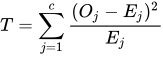
- where Oj are observed counts, Ej are corresponding expected count and c is the number of classes for which counts/frequencies are being analysed.
The test statistic is distributed approximately as a chi-square random variable with c-1 degrees of freedom. The test has relatively low power (chance of detecting a real effect) with all but large numbers or big deviations from the null hypothesis (all classes contain observations that could have been in those classes by chance).
The handling of small expected frequencies is controversial. Koehler and Larntz (1980) assert that the chi-square approximation is adequate provided all of the following are true:
- total of observed counts (N) ≥ 10
- number of classes (c) ≥ 3
- all expected values ≥ 0.25
Some statistical software offers exact methods for dealing with small frequencies but these methods are not appropriate for all expected distributions, hence they can be specious. You can try reducing the number of classes but expert statistical guidance is advisable for this (Conover, 1999).
Example
Suppose we suspected an unusual distribution of blood groups in patients undergoing one type of surgical procedure. We know that the expected distribution for the population served by the hospital which performs this surgery is 44% group O, 45% group A, 8% group B and 3% group AB. We can take a random sample of routine pre-operative blood grouping results and compare these with the expected distribution.
Results for 187 consecutive patients:
| Blood Group: | O | 67 |
| A | 83 | |
| B | 29 | |
| AB | 8 |
To analyse these data using StatsDirect you must first enter the observed frequencies into a workbook column, as above, and enter the expected distribution in another column of the same length: proportions, percentages or expected counts, which are scaled to the observed total (for this example the percentages 44, 45, 8 and 3). A third column may hold the names of the categories. Then choose Chi-square Goodness of Fit from the Nonparametric section of the analysis menu and select the observed column, the expected column, and the names or skip them. The expected frequencies are calculated and displayed; the degrees of freedom are the number of categories minus one. The results for our example are:
N = 187
| Value | Observed frequency | Expected frequency |
| 1 | 67 | 82.28 |
| 2 | 83 | 84.15 |
| 3 | 29 | 14.96 |
| 4 | 8 | 5.61 |
Chi-square = 17.048101 df = 3
P = 0.0007
Here we may report a statistically highly significant difference between the distribution of blood groups from patients undergoing this surgical procedure and that which would be expected from a random sample of the general population.
You can then ask for a simulated exact P value (Simulate Exact P): the observed total is drawn again and again from the expected distribution, and the P value is the proportion of the draws whose chi-square is at least that of your table; it is given with an exact (Clopper-Pearson) confidence interval for that proportion. Frequencies that are not whole numbers are used as you entered them by the test; they are rounded to the nearest whole number for the simulation, and the results say when this has been done.

 R code
This R code reproduces the example above. It needs no packages and was checked with R 4.6.1. Paste it into R, or save it as a script and run it.
# Chi-square goodness of fit: the StatsDirect help example (blood groups of 187
# consecutive patients against the distribution expected in the population) in R
observed <- c(O = 67, A = 83, B = 29, AB = 8)
expected <- c(0.44, 0.45, 0.08, 0.03)     # proportions expected; they add up to 1

# R's standard test. With p given it compares the counts with those proportions;
# rescale.p = TRUE lets p be percentages or expected counts instead.
test <- chisq.test(observed, p = expected)
print(test)

# Observed and expected frequencies, and the result as StatsDirect reports it
cat("N =", sum(observed), "\n")
print(cbind("Observed frequency" = observed, "Expected frequency" = test$expected))
cat(sprintf("Chi-square = %.6f  df = %d\nP = %.4f\n", test$statistic,
            test$parameter, test$p.value))

# Like StatsDirect, R warns when the expected frequencies are small: the
# chi-square approximation is then unreliable.