Unpaired (Two Sample) t Test
Menu location: Analysis_Parametric_Unpaired t.
This function gives an unpaired two sample Student t test with a confidence interval for the difference between the means.
The unpaired t method tests the null hypothesis that the population means related to two independent, random samples from an approximately normal distribution are equal (Altman, 1991; Armitage and Berry, 1994).
Assuming equal variances, the test statistic is calculated as:
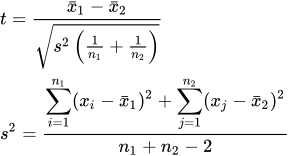
- where x bar 1 and x bar 2 are the sample means, s² is the pooled sample variance, n1 and n2 are the sample sizes and t is a Student t quantile with n1 + n2 - 2 degrees of freedom.
Power is calculated as the power achieved with the given sample sizes and variances for detecting the observed difference between means with a two-sided type I error probability of (100-CI%)% (Dupont, 1990).
The unpaired t test should not be used if there is a significant difference between the variances of the two samples; StatsDirect tests for this and gives appropriate warnings. For the situation of unequal variances, StatsDirect calculates Satterthwaite's approximate t test; a method in the Behrens-Welch family (Armitage and Berry, 1994).
Assuming unequal variances, the test statistic is calculated as:
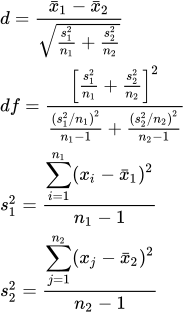
- where x bar 1 and x bar 2 are the sample means, s² is the sample variance, n1 and n2 are the sample sizes, d is the Behrens-Welch test statistic evaluated as a Student t quantile with df degrees of freedom using Satterthwaite's approximation.
Note that the nonparametric Mann-Whitney test is not a remedy for unequal variances; use the unequal variances t test above.
Example
From Armitage and Berry (1994, p. 111).
Test workbook (Parametric worksheet: Low Protein, High Protein).
Consider the gain in weight of 19 female rats between 28 and 84 days after birth. 12 were fed on a high protein diet and 7 on a low protein diet.
| High protein | Low protein |
| 134 | 70 |
| 146 | 118 |
| 104 | 101 |
| 119 | 85 |
| 124 | 107 |
| 161 | 132 |
| 107 | 94 |
| 83 | |
| 113 | |
| 129 | |
| 97 | |
| 123 |
To analyse these data in StatsDirect first prepare them in two workbook columns and label these columns appropriately. Alternatively, open the test workbook using the file open function of the file menu. Then select the unpaired t test from the parametric methods section of the analysis menu. Select the columns marked "High protein" and "Low protein" when prompted for data.
For this example:
Unpaired t test
Mean of High Protein = 120 (n = 12)
Mean of Low Protein = 101 (n = 7)
Assuming equal variances
Combined standard error = 10.045276
df = 17
t = 1.891436
One sided P = 0.0379
Two sided P = 0.0757
95% confidence interval for difference between means = -2.193679 to 40.193679
Power (for 5% significance) = 43.05%
Assuming unequal variances
Combined standard error = 9.943999
df = 13.081702
t(d) = 1.9107
One sided P = 0.0391
Two sided P = 0.0782
95% confidence interval for difference between means = -2.469073 to 40.469073
Power (for 5% significance) = 42.49%
Comparison of variances
Two sided F test is not significant
No need to assume unequal variances
Thus we have a difference that is not quite significant at the 5% level. The most important information is, however, conveyed by the confidence interval. The 95% CI includes zero therefore we can not be confident (at the 95% level) that these data show any difference in weight gain. As most of the interval is toward weight gain and as the test result is in the grey "suggestive" 5%-10% zone we have good evidence for repeating this experiment with larger numbers. Bigger samples will probably shrink the range of uncertainty so that the confidence interval contracts to a narrower band that excludes zero.
N.B. We did not consider a one sided P value here because we could not be absolutely certain that the rats would all benefit from a high protein diet in comparison with those on a low protein diet.

 R code
This R code reproduces the example above. It needs no packages and was checked with R 4.6.1. Paste it into R, or save it as a script and run it.
# Unpaired t test: the StatsDirect help example (Armitage and Berry 1994, weight
# gain of 19 rats on high or low protein diets) in R
high <- c(134, 146, 104, 119, 124, 161, 107, 83, 113, 129, 97, 123)
low <- c(70, 118, 101, 85, 107, 132, 94)

# R's standard test, first assuming equal variances and then not (R's default,
# the Welch test, whose t and df are StatsDirect's t(d) and its fractional df).
# Each gives t, df, the two sided P and the confidence interval.
equal <- t.test(high, low, var.equal = TRUE)
print(equal)
unequal <- t.test(high, low)
print(unequal)

# The F test that StatsDirect uses to compare the variances
f <- var.test(high, low)
print(f)

# The report's other lines, to 6 decimal places
six <- function(x) formatC(x, digits = 6, format = "f", drop0trailing = TRUE)
cat(sprintf("Mean of High Protein = %s  (n = %d)\n", six(mean(high)), length(high)))
cat(sprintf("Mean of Low Protein = %s  (n = %d)\n", six(mean(low)), length(low)))
delta <- mean(high) - mean(low)
report <- function(r, label, t) {
  cat(label, "\n")
  cat("Combined standard error =", six(delta / r$statistic), "  df =",
      six(r$parameter), " ", t, "=", six(r$statistic), "\n")
  cat(sprintf("One sided P = %.4f   Two sided P = %.4f\n", r$p.value / 2, r$p.value))
  cat("95% confidence interval for difference between means =", six(r$conf.int[1]),
      "to", six(r$conf.int[2]), "\n")
  # Power of a two sided test at the 5% level to detect the difference seen, from
  # the noncentral t distribution: the noncentrality parameter is the t observed
  tc <- qt(0.975, r$parameter)
  pw <- pt(-tc, r$parameter, ncp = r$statistic) +
        pt(tc, r$parameter, ncp = r$statistic, lower.tail = FALSE)
  cat(sprintf("Power (for 5%% significance) = %.2f%%\n", 100 * pw))
}
report(equal, "Assuming equal variances", "t")
report(unequal, "Assuming unequal variances", "t(d)")
cat("Two sided F test is", if (f$p.value < 0.05) "significant" else "not significant",
    "\n")