Direct Standardization
Menu location: Analysis_Rates_Direct Standardization.
This function calculates directly standardized rates (DSR) with approximate confidence intervals.
DSR is simply a weighted mean event rate for a study population, using the group/stratum sizes of a reference population as the weighting scheme. Standardized or adjusted rates are summary index measures for the purpose of comparison only; their magnitude has no intrinsic value.
The choice of a reference or standard population is important; it must relate to the population under study naturally.
Please note that standardization is not a substitute for individual comparisons of stratum-specific rates.
This method is unreliable with small numbers; there should be at least 25 events observed overall and at least one event in each stratum. If the number of events is small, consider aggregating strata.
Direct standardization is not appropriate if there is not a consistent relationship between stratum-specific rates in different populations being compared.
There are a lot of pitfalls in using directly standardized rates; if you have any doubts then please consult with an Epidemiologist and/or Statistician.
Data input
- Number of events for each group from the index/study population
- Person-time for each group from the index/study population (e.g. size of each group if just one year and all subjects were followed up)
- Group sizes or weights from a reference/standard population
- Group/stratum labels, e.g. age bands
Note that an alternative binomial method is provided for situations where your observed rates are too large for the Poisson distribution to be used, namely one or more rates r are not so small that 1-r can be considered almost equal to 1.
Technical validation
Approximate confidence intervals for the DSR are calculated firstly by Chiang's normal approximation to Poisson rate sums (Chiang, 1961; Keyfitz, 1966; Breslow and Day, 1987; Armitage and Berry, 1994) and secondly by an improved approximation adjusted for the total number of observed events (Dobson et al., 1991).
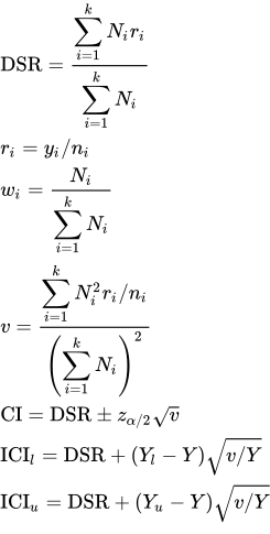
- where v is the approximate (Chiang) variance, wi is the reference weight for the ith stratum, ri is the observed study rate for the ith stratum, Ni is the reference population size for the ith stratum, yi is the number of events observed in the ith stratum of the study population, ni is the person-time for the ith stratum of the study population, zα/2 is the 100(1 - α/2) centile of the standard normal distribution, Y is the total number of events observed, Yl and Yu are the exact lower and upper confidence limits for the Poisson count Y and ICI l to u is the improved confidence interval due to Dobson et al. For large rates, the binomial variance is used, where r(1-r) is substituted for r in the variance formula above.
Example
From Curtin and Klein (1995):
Test workbook (Rates worksheet: Age Bands, Index Events, Index Group Sizes, Reference Sizes).
The following data relate to stroke deaths for males from a hypothetical medium-size US State. The reference population is the 1940 US Standard Million.
| Age group | Deaths | Person-Time (thousands) | Reference Size/Weight |
| Under 1 | 1 | 38 | 15343 |
| 1-4 | 0 | 150 | 64718 |
| 5-14 | 1 | 322 | 170355 |
| 15-24 | 2 | 344 | 181677 |
| 25-34 | 8 | 443 | 162066 |
| 35-44 | 21 | 379 | 139237 |
| 45-54 | 46 | 256 | 117811 |
| 55-64 | 103 | 189 | 80294 |
| 65-74 | 254 | 136 | 48426 |
| 75-84 | 371 | 57 | 17303 |
| 85 and over | 212 | 12 | 2770 |
To analyse these data in StatsDirect you must select direct standardization from the rates section of the analysis menu. Note that annual mortality rates are often expressed as rates per 100,000 population or units of person time (i.e. 100,000 person years); so a multiplier of 100,000 should be selected for the scaling of rates in the output - you are prompted to provide this.
For this example:
Directly Standardized Rates
Rates are expressed per 100000 units of person time:
| Index events | Index PT | Index rate | Reference size | Weight |
| 1 | 38000 | 2.631579 | 15343 | 0.015343 |
| 0 | 150000 | 0 | 64718 | 0.064718 |
| 1 | 322000 | 0.310559 | 170355 | 0.170355 |
| 2 | 344000 | 0.581395 | 181677 | 0.181677 |
| 8 | 443000 | 1.805869 | 162066 | 0.162066 |
| 21 | 379000 | 5.540897 | 139237 | 0.139237 |
| 46 | 256000 | 17.96875 | 117811 | 0.117811 |
| 103 | 189000 | 54.497354 | 80294 | 0.080294 |
| 254 | 136000 | 186.764706 | 48426 | 0.048426 |
| 371 | 57000 | 650.877193 | 17303 | 0.017303 |
| 212 | 12000 | 1766.666667 | 2770 | 0.00277 |
| Index rate | Exact 95% confidence interval | |
| 2.631579 | 0.066626 to 14.662219 | Under 1 year |
| 0 | 0 to 2.459253 | 1-4 years |
| 0.310559 | 0.007863 to 1.730324 | 5-14 years |
| 0.581395 | 0.07041 to 2.1002 | 15-24 years |
| 1.805869 | 0.779646 to 3.558282 | 25-34 years |
| 5.540897 | 3.429903 to 8.46985 | 35-44 years |
| 17.96875 | 13.155383 to 23.967794 | 45-54 years |
| 54.497354 | 44.482507 to 66.093892 | 55-64 years |
| 186.764706 | 164.500721 to 211.201647 | 65-74 years |
| 650.877193 | 586.323368 to 720.597325 | 75-84 years |
| 1766.666667 | 1536.8427 to 2021.164948 | 85 years and over |
Total events = 1019
Adjusted events = 766.55342
Crude rate = 43.809114
Adjusted rate R = 32.955865
Any rates (binomial model)
Approximate standard error of R = 1.050864
Approximate 95% confidence interval = 30.89621 to 35.01552
Small rates (Poisson model)
Approximate standard error of R = 1.053213
Approximate 95% confidence interval = 30.891605 to 35.020125
Improved approximate (Dobson) 95% confidence interval = 30.923031 to 35.085201

 R code
This R code reproduces the example above. It needs no packages and was checked with R 4.6.1. Paste it into R, or save it as a script and run it.
# Direct standardization: the StatsDirect help example (Curtin and Klein 1995, stroke
# deaths in males of a hypothetical US state, standardized to the 1940 US Standard
# Million; the test workbook's Rates worksheet columns Age Bands, Index Events, Index
# Group Sizes and Reference Sizes) in R
age <- c("Under 1 year", "1-4 years", "5-14 years", "15-24 years", "25-34 years",
         "35-44 years", "45-54 years", "55-64 years", "65-74 years", "75-84 years",
         "85 years and over")
deaths <- c(1, 0, 1, 2, 8, 21, 46, 103, 254, 371, 212)
# person-time in person-years (the table above gives thousands)
person_time <- c(38000, 150000, 322000, 344000, 443000, 379000, 256000, 189000,
                 136000, 57000, 12000)
reference <- c(15343, 64718, 170355, 181677, 162066, 139237, 117811, 80294, 48426,
               17303, 2770)
per <- 100000   # the multiplier chosen for the rates
conf <- 0.95

six <- function(x) formatC(x, digits = 6, format = "f", drop0trailing = TRUE)

# Base R has no direct standardization function, so the rate is computed as the
# formulae above give it: the stratum rates weighted by the reference population
rate <- deaths / person_time
weight <- reference / sum(reference)
cat("Rates are expressed per", format(per, scientific = FALSE),
    "units of person time:\n")
cat("Index events  Index PT  Index rate  Reference size  Weight\n")
for (i in seq_along(age)) {
  cat(deaths[i], person_time[i], six(rate[i] * per), reference[i], six(weight[i]),
      "\n")
}

# The exact confidence interval for each stratum's Poisson count over its person-time
# is what poisson.test() gives (its conf.int)
# (poisson.test() takes whole-number counts; qgamma(0.025, y) and qgamma(0.975, y + 1)
# over the person-time give the same limits for fractional counts)
cat("Index rate  Exact 95% confidence interval\n")
for (i in seq_along(age)) {
  ci <- poisson.test(deaths[i], person_time[i], conf.level = conf)$conf.int * per
  cat(six(rate[i] * per), six(ci[1]), "to", six(ci[2]), age[i], "\n")
}

# The directly standardized rate and, applied to the study's person-time, the number of
# events it would have had at the standardized rate
total <- sum(deaths)
dsr <- sum(weight * rate)
cat("Total events =", total, "\n")
cat("Adjusted events =", six(dsr * sum(person_time)), "\n")
cat("Crude rate =", six(total / sum(person_time) * per), "\n")
cat("Adjusted rate R =", six(dsr * per), "\n")

# The variance of the rate as a weighted sum of binomial proportions (any rates) and
# as a weighted sum of Poisson rates (Chiang 1961, small rates), each with a normal
# interval; a stratum whose rate is 0 or 1 adds nothing to the binomial variance
z <- qnorm(1 - (1 - conf) / 2)
v_binomial <- sum(weight^2 * rate * (1 - rate) / person_time)
v_poisson <- sum(weight^2 * rate / person_time)
cat("Any rates (binomial model)\n")
cat("Approximate standard error of R =", six(sqrt(v_binomial) * per), "\n")
cat("Approximate 95% confidence interval =", six((dsr - z * sqrt(v_binomial)) * per),
    "to", six((dsr + z * sqrt(v_binomial)) * per), "\n")
cat("Small rates (Poisson model)\n")
cat("Approximate standard error of R =", six(sqrt(v_poisson) * per), "\n")
cat("Approximate 95% confidence interval =", six((dsr - z * sqrt(v_poisson)) * per),
    "to", six((dsr + z * sqrt(v_poisson)) * per), "\n")

# Dobson et al. (1991): the exact limits for the total count of events, shifted and
# scaled to the standardized rate
total_ci <- poisson.test(total, conf.level = conf)$conf.int
dobson <- dsr + (total_ci - total) * sqrt(v_poisson / total)
cat("Improved approximate (Dobson) 95% confidence interval =",
    six(dobson[1] * per), "to", six(dobson[2] * per), "\n")