Grouped Linear Regression with Covariance Analysis
Menu location: Analysis_Regression and Correlation_Grouped Linear_Covariance.
This function compares the slopes and separations of two or more simple linear regression lines.
The method involves examination of regression parameters for a group of xY pairs in relation to a common fitted function. This provides an analysis of variance that shows whether or not there is a significant difference between the slopes of the individual regression lines as a whole. StatsDirect then compares all of the slopes individually. The vertical distance between each regression line is then examined using analysis of covariance and the corrected means are given (Armitage and Berry, 1994).
Assumptions:
- Y replicates are a random sample from a normal distribution
- deviations from the regression line (residuals) follow a normal distribution
- deviations from the regression line (residuals) have uniform variance
This is just one facet of analysis of covariance; there are additional and alternative methods. For further information, see Kleinbaum et al. (1998) and Armitage and Berry (1994). Analysis of covariance is best carried out as part of a broader regression modelling exercise by a Statistician.
Technical Validation
Slopes of several regression lines are compared by analysis of variance as follows (Armitage, 1994):

- where SScommon is the sum of squares due to the common slope of k regression lines, SSbetween is the sum of squares due to differences between the slopes, SStotal is the total sum of squares and the residual sum of squares is the difference between SStotal and SScommon. Sxxj is the sum of squares about the mean x observation in the jth group, SxYj is the sum of products of the deviations of xY pairs from their means in the jth group and SYYj is the sum of squares about the mean Y observation in the jth group.
Vertical separation of slopes of several regression lines is tested by analysis of covariance as follows (Armitage, 1994):
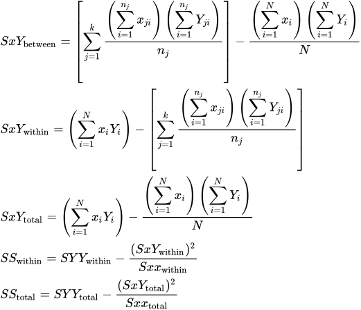
- where SS are corrected sums of squares within the groups, total and between the groups (subtract within from total). The constituent sums of products or squares are partitioned between groups, within groups and total as above.
Data preparation
If there are equal numbers of replicate Y observations or single Y observations for each x then you are best prepare and select your data using a group identifier variable. For example with three replicates you would prepare five columns of data: group identifier, x, y1, y2, and y3. Remember to choose the "Groups by identifier" option in this case.
If there are unequal numbers of replicate Y observations for each x then you must prepare the x data in separate columns by group, prepare the Y data in separate columns by group and observation (i.e. Y for group 1 observation 1… r rows long where r is the number of repeat observations). Remember to choose the "Groups by column" option in this case. This is done in the example below.
Example
From Armitage and Berry (1994).
Test workbook (Regression worksheet: Log Dose_Std, BD 1_Std, BD 2_Std, BD 3_Std, Log Dose_I, BD 1_I, BD 2_I, BD 3_I, Log Dose_F, BD 1_F, BD 2_F, BD 3_F).
Three different preparations of Vitamin D are tested for their effect on bones by feeding them to rats that have an induced lack of mineral in their bones. X-ray methods are used to test the re-mineralisation of bones in response to the Vitamin D.
For the standard preparation:
|
Log dose of Vit D |
||
|
0.544 |
0.845 |
1.146 |
|
Bone density score |
||
|
0 |
1.5 |
2 |
|
0 |
2.5 |
2.5 |
|
1 |
5 |
5 |
|
2.75 |
6 |
4 |
|
2.75 |
4.25 |
5 |
|
1.75 |
2.75 |
4 |
|
2.75 |
1.5 |
2.5 |
|
2.25 |
3 |
3.5 |
|
2.25 |
|
3 |
|
2.5 |
|
2 |
|
|
|
3 |
|
|
|
4 |
|
|
|
4 |
For alternative preparation I:
| Log dose of Vit D | ||||
| 0.398 | 0.699 | 1.000 | 1.301 | 1.602 |
| Bone density score | ||||
| 0 | 1 | 1.5 | 3 | 3.5 |
| 1 | 1.5 | 1 | 3 | 3.5 |
| 0 | 1.5 | 2 | 5.5 | 4.5 |
| 0 | 1 | 3.5 | 2.5 | 3.5 |
| 0 | 1 | 2 | 1 | 3.5 |
| 0.5 | 0.5 | 0 | 2 | 3 |
For alternative preparation F:
| Log dose of Vit D | ||
| 0.398 | 0.699 | 1.000 |
| Bone density score | ||
| 2.75 | 2.5 | 3.75 |
| 2 | 2.75 | 5.25 |
| 1.25 | 2.25 | 6 |
| 2 | 2.25 | 5.5 |
| 0 | 3.75 | 2.25 |
| 0.5 | 3.5 | |
To analyse these data in StatsDirect you must first enter them into 14 columns in the workbook appropriately labelled. The first column is just three rows long and contains the three log doses of vitamin D for the standard preparation. The next three columns represent the repeated measures of bone density for each of the three levels of log dose of vitamin D which are represented by the rows of the first column. This is then repeated for the other two preparations. Alternatively, open the test workbook using the file open function of the file menu. Then select covariance from the groups section of the regression and correlation section of the analysis menu. Select the columns marked "Log Dose_Std", "Log Dose_I" and "Log Dose_F" when you are prompted for the predictor (x) variables, these contain the log dose levels (logarithms are taken because, from previous research, the relationship between bone re-mineralisation and Vitamin D is known to be log-linear). Make sure that the "use Y replicates" option is checked when you are prompted for it. Then select the outcome (Y) variables that represent the replicates. You will have to select three, five and three columns in just three selection actions because these are the number of corresponding dose levels in the x variables in the order in which you selected them.
Alternatively, these data could have been entered in just three pairs of workbook columns representing the three preparations with a log dose column and column of the mean bone density score for each dose level. By accepting the more long winded input of replicates, StatsDirect is encouraging you to run a test of linearity on your data.
For this example:
Grouped linear regression
| Source of variation | SSq | DF | MSq | VR | |
| Common slope | 78.340457 | 1 | 78.340457 | 67.676534 | P < 0.0001 |
| Between slopes | 4.507547 | 2 | 2.253774 | 1.946984 | P = 0.1501 |
| Separate residuals | 83.34518 | 72 | 1.157572 | ||
| Within groups | 166.193185 | 75 |
Common slope is significant
Difference between slopes is NOT significant
Slope comparisons:
slope 1 (Log Dose_Std) v slope 2 (Log Dose_I) = 2.616751 v 2.796235
Difference (95% CI) = 0.179484 (-1.576065 to 1.935032)
t = -0.203808, P = 0.8391
slope 1 (Log Dose_Std) v slope 3 (Log Dose_F) = 2.616751 v 4.914175
Difference (95% CI) = 2.297424 (-0.245568 to 4.840416)
t = -1.800962, P = 0.0759
slope 2 (Log Dose_I) v slope 3 (Log Dose_F) = 2.796235 v 4.914175
Difference (95% CI) = 2.11794 (-0.135343 to 4.371224)
t = -1.873726, P = 0.065
Covariance analysis
Uncorrected:
| Source of variation | YY | xY | xx | DF |
| Between groups | 17.599283 | -3.322801 | 0.988515 | 2 |
| Within | 166.193185 | 25.927266 | 8.580791 | 75 |
| Total | 183.792468 | 22.604465 | 9.569306 | 77 |
Corrected:
| Source of variation | SSq | DF | MSq | VR |
| Between groups | 42.543829 | 2 | 21.271915 | 17.917733 |
| Within | 87.852727 | 74 | 1.187199 | |
| Total | 130.396557 | 76 |
P < 0.0001
Corrected Y means ± SE for baseline mean predictor of 0.884372:
Y' = 2.901917 ± 0.195733
Y' = 1.533957 ± 0.203527
Y' = 3.398345 ± 0.273111
Line separations (common slope =3.021547):
line 1 (Log Dose_Std) vs line 2 (Log Dose_I) Vertical separation = 1.367959
95% CI = 0.804164 to 1.931754
t = 4.834592, (74 df), P < 0.0001
line 1 (Log Dose_Std) vs line 3 (Log Dose_F) Vertical separation = -0.496428
95% CI = -1.164377 to 0.171521
t = -1.480883, (74 df), P = 0.1429
line 2 (Log Dose_I) vs line 3 (Log Dose_F) Vertical separation = -1.864388
95% CI = -2.560193 to -1.168583
t = -5.338959, (74 df), P < 0.0001
The common slope is highly significant and the test for difference between the slopes overall was non-significant. If our assumption of linearity holds true we can conclude that these lines are reasonably parallel. Looking more closely at the individual slopes preparation F is almost shown to be significantly different from the other two but this difference was not large enough to throw the overall slope comparison into a significant heterogeneity.
The analysis of covariance shows a highly significant vertical separation of the lines: at a given log dose, preparation I gave lower bone density scores than the standard and than preparation F, while the standard and preparation F did not differ significantly. (Earlier versions of StatsDirect counted the degrees of freedom of this analysis from the dose levels rather than the rats when the scores were entered as replicates, and found no separation.)

 R code
This R code reproduces the example above. It needs no packages and was checked with R 4.6.1. Paste it into R, or save it as a script and run it.
# Grouped linear regression with covariance analysis: the StatsDirect help example
# (Armitage and Berry 1994, bone density of rats given three preparations of
# vitamin D at several log doses, with replicate scores at each dose; the test
# workbook's columns Log Dose_Std, BD 1_Std to BD 3_Std, Log Dose_I, BD 1_I to
# BD 5_I, Log Dose_F and BD 1_F to BD 3_F) in R
std <- list(x = c(0.544, 0.845, 1.146),
            y = list(c(0, 0, 1, 2.75, 2.75, 1.75, 2.75, 2.25, 2.25, 2.5),
                     c(1.5, 2.5, 5, 6, 4.25, 2.75, 1.5, 3),
                     c(2, 2.5, 5, 4, 5, 4, 2.5, 3.5, 3, 2, 3, 4, 4)))
prep_i <- list(x = c(0.398, 0.699, 1, 1.301, 1.602),
               y = list(c(0, 1, 0, 0, 0, 0.5), c(1, 1.5, 1.5, 1, 1, 0.5),
                        c(1.5, 1, 2, 3.5, 2, 0), c(3, 3, 5.5, 2.5, 1, 2),
                        c(3.5, 3.5, 4.5, 3.5, 3.5, 3)))
prep_f <- list(x = c(0.398, 0.699, 1),
               y = list(c(2.75, 2, 1.25, 2, 0, 0.5), c(2.5, 2.75, 2.25, 2.25, 3.75),
                        c(3.75, 5.25, 6, 5.5, 2.25, 3.5)))
groups <- list("Log Dose_Std" = std, "Log Dose_I" = prep_i, "Log Dose_F" = prep_f)

# One row per rat: its group, log dose and score
d <- do.call(rbind, lapply(names(groups), function(g) {
  data.frame(group = g, x = rep(groups[[g]]$x, lengths(groups[[g]]$y)),
             y = unlist(groups[[g]]$y))
}))
d$group <- factor(d$group, levels = names(groups))

# R's standard comparison of the regression lines: separate lines against a
# common slope (the "group:x" line is the between slopes test) and the common
# slope itself, each against the residual about the separate lines
separate <- lm(y ~ group * x, data = d)
print(anova(lm(y ~ group + x, data = d), separate))
print(anova(separate))

# The report's table to 6 places: the common slope, the difference between the
# slopes, the residual about the separate lines and the within groups total
six <- function(x) formatC(x, digits = 6, format = "f", drop0trailing = TRUE)
pv <- function(p) {
  if (p < 0.0001) "P < 0.0001" else
    paste("P =", formatC(p, digits = 4, format = "f", drop0trailing = TRUE))
}
a <- anova(separate)
ss_common <- a["x", "Sum Sq"]
ss_between <- a["group:x", "Sum Sq"]
ss_res <- a["Residuals", "Sum Sq"]
df_res <- a["Residuals", "Df"]
ms_res <- ss_res / df_res
cat("Common slope", six(ss_common), 1, six(ss_common), six(ss_common / ms_res),
    pv(pf(ss_common / ms_res, 1, df_res, lower.tail = FALSE)), "\n")
vr_between <- ss_between / 2 / ms_res
cat("Between slopes", six(ss_between), 2, six(ss_between / 2), six(vr_between),
    pv(pf(vr_between, 2, df_res, lower.tail = FALSE)), "\n")
cat("Separate residuals", six(ss_res), df_res, six(ms_res), "\n")
within <- sum(tapply(d$y, d$group, function(v) sum((v - mean(v))^2)))
cat("Within groups", six(within), nrow(d) - 3, "\n")

# Each pair of slopes: their difference with its confidence interval and t test on
# the residual mean square about the separate lines
slope <- function(g) coef(lm(y ~ x, data = d[d$group == g, ]))[2]
ssx <- function(g) with(d[d$group == g, ], sum((x - mean(x))^2))
tcrit <- qt(0.975, df_res)
for (pair in list(1:2, c(1, 3), 2:3)) {
  g1 <- names(groups)[pair[1]]
  g2 <- names(groups)[pair[2]]
  se <- sqrt(ms_res * (1 / ssx(g1) + 1 / ssx(g2)))
  dif <- abs(slope(g1) - slope(g2))
  t <- (slope(g1) - slope(g2)) / se
  cat("slope", pair[1], "(", g1, ") v slope", pair[2], "(", g2, ") =",
      six(slope(g1)), "v", six(slope(g2)), "\n")
  cat("  Difference (95% CI) =", six(dif), "(", six(dif - tcrit * se), "to",
      six(dif + tcrit * se), ")  t =", six(t), " ", pv(2 * pt(-abs(t), df_res)), "\n")
}

# The covariance analysis compares the groups at the same log dose, with the lines
# made parallel. The uncorrected table holds the sums of squares and products of
# the scores (YY), the products with log dose (xY) and the log doses (xx): between
# the groups, within them and in total, over every rat
k <- 3
n_g <- table(d$group)
sy_g <- tapply(d$y, d$group, sum)
sx_g <- tapply(d$x, d$group, sum)
syy_b <- sum(sy_g^2 / n_g) - sum(d$y)^2 / nrow(d)
sxx_b <- sum(sx_g^2 / n_g) - sum(d$x)^2 / nrow(d)
sxy_b <- sum(sx_g * sy_g / n_g) - sum(d$x) * sum(d$y) / nrow(d)
syy_t <- sum((d$y - mean(d$y))^2)
sxx_t <- sum((d$x - mean(d$x))^2)
sxy_t <- sum((d$x - mean(d$x)) * (d$y - mean(d$y)))
cat("Uncorrected: Between groups", six(syy_b), six(sxy_b), six(sxx_b), k - 1, "\n")
cat("Uncorrected: Within", six(syy_t - syy_b), six(sxy_t - sxy_b), six(sxx_t - sxx_b),
    nrow(d) - k, "\n")
cat("Uncorrected: Total", six(syy_t), six(sxy_t), six(sxx_t), nrow(d) - 1, "\n")

# The corrected table is R's comparison of the parallel lines model with a single
# line: the drop in residual sum of squares is the between groups sum of squares,
# and the parallel lines model's residual is the corrected within groups sum
common <- lm(y ~ x, data = d)
parallel <- lm(y ~ x + group, data = d)
print(anova(common, parallel))
cv <- anova(common, parallel)
css_w <- cv$RSS[2]
df_w <- cv$Res.Df[2]
css_b <- cv$"Sum of Sq"[2]
vr <- (css_b / (k - 1)) / (css_w / df_w)
cat("Corrected: Between groups", six(css_b), k - 1, six(css_b / (k - 1)), six(vr), "\n")
cat("Corrected: Within", six(css_w), df_w, six(css_w / df_w), "\n")
cat("Corrected: Total", six(cv$RSS[1]), cv$Res.Df[1], "\n")
cat(pv(pf(vr, k - 1, df_w, lower.tail = FALSE)), "\n")

# Corrected means: each group's line at the mean log dose of all the rats, with
# the standard error R gives for a prediction from the parallel lines model
mx0 <- mean(d$x)
at_mean <- predict(parallel, newdata = data.frame(x = mx0, group = names(groups)),
                   se.fit = TRUE)
cat("Corrected Y means +/- SE for baseline mean predictor of", six(mx0), ":\n")
for (g in 1:3) cat("  Y' =", six(at_mean$fit[g]), "+/-", six(at_mean$se.fit[g]), "\n")

# The vertical separations of the lines are the differences between the group
# terms of the parallel lines model (the first group is the baseline, so its
# term is zero), with their standard errors from the model's covariance matrix
bs <- coef(parallel)["x"]
cat("Line separations (common slope =", six(bs), "):\n")
term <- c(0, coef(parallel)[c("groupLog Dose_I", "groupLog Dose_F")])
v <- matrix(0, 3, 3)
v[2:3, 2:3] <- vcov(parallel)[c("groupLog Dose_I", "groupLog Dose_F"),
                              c("groupLog Dose_I", "groupLog Dose_F")]
tcrit <- qt(0.975, df_w)
for (pair in list(1:2, c(1, 3), 2:3)) {
  g1 <- pair[1]
  g2 <- pair[2]
  sep <- term[g1] - term[g2]
  se <- sqrt(v[g1, g1] + v[g2, g2] - 2 * v[g1, g2])
  cat("  line", g1, "vs line", g2, "Vertical separation =", six(sep), " 95% CI =",
      six(sep - tcrit * se), "to", six(sep + tcrit * se), " t =", six(sep / se),
      paste0("(", df_w, " df)"), pv(2 * pt(-abs(sep / se), df_w)), "\n")
}

# The report ends with a plot of the scores against log dose with the three fitted
# lines
plot(d$x, d$y, pch = as.numeric(d$group), col = as.numeric(d$group),
     xlab = "Log Dose_Std Log Dose_I Log Dose_F", ylab = "Y Replicates",
     main = "Grouped linear regression")
for (g in 1:3) abline(lm(y ~ x, data = d[d$group == names(groups)[g], ]), col = g)
legend("bottomright", legend = names(groups), pch = 1:3, col = 1:3, bty = "n")