Linearized Estimates
Menu location: Analysis_Regression and Correlation_Linearized Estimates.
This section provides simple (one predictor) regression estimates for three linearized functions (exponential, geometric and hyperbolic) by an unweighted least squares method.
These functions should be used only to indicate that a more robust fit of the selected model is worth investigating with your data.
Exponential
Data are linearized by logarithmic transformation of the outcome (Y) variable. Simple linear regression of ln(Y) vs. x gives ln(a) as the intercept and b as the slope for the function: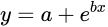
Geometric
Data are linearized by logarithmic transformation of both variables. Simple linear regression of ln(Y) vs. ln(x) gives ln(a) as the intercept and b as the slope for the function: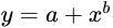
Hyperbolic
Data are linearized by reciprocal transformation of both variables. Simple linear regression of 1/Y vs. 1/x gives a as the slope and b as the intercept for the function: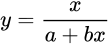
The standard error of the estimate is given for each of these regressions but please note that the errors of your outcome/response variable might not be from a normal distribution.
This section of StatsDirect is intended only for those who are familiar with regression modelling and who use these linearized estimates as a springboard for further modelling. Generic modelling software such as R, S+ or GLIMM can be used for further modelling, which is best done by a Statistician.
Example
An illustration with the electricity consumption and home size data of the polynomial regression example (McClave and Dietrich, 1991).
Test workbook (Regression worksheet: Home Size, KW Hrs/Mnth).
Select Linearized Estimates from the Regression and Correlation section of the analysis menu, choose each model in turn, and select the columns marked "KW Hrs/Mnth" and "Home Size" when asked for the outcome and predictor.
For this example:
Linearized Estimates
Model : (Exponential) Y = a * exp(b * x)
Method: unweighted least squares
For KW Hrs/Mnth vs Home Size
A = 816.912669
B = 0.000346
Correlation coefficient (r) = 0.892077 (r² = 0.795802)
Standard error of estimate = 0.09634
Model : (Geometric / Power) Y = a * x^b
Method: unweighted least squares
For KW Hrs/Mnth vs Home Size
A = 7.27571
B = 0.715637
Correlation coefficient (r) = 0.938647 (r² = 0.881058)
Standard error of estimate = 0.073527
Model : (Hyperbolic) Y = x / (a + b * x)
Method: unweighted least squares
For KW Hrs/Mnth vs Home Size
A = 0.907439
B = 0.000137
Correlation coefficient (r) = 0.957812 (r² = 0.917405)
Standard error of estimate = 0.000041
The hyperbolic model fits these data best of the three on its own scale, but the standard errors are on different scales and none of the models should be used beyond the observed home sizes: these estimates suggest which non-linear model might be worth fitting properly.

 R code
This R code reproduces the illustration above. It needs no packages and was checked with R 4.6.1. Paste it into R, or save it as a script and run it.
# Linearized regression estimates: an illustration with the electricity
# consumption and home size data of the polynomial regression topic (McClave and
# Dietrich 1991, the test workbook's Home Size and KW Hrs/Mnth) in R
size <- c(1290, 1350, 1470, 1600, 1710, 1840, 1980, 2230, 2400, 2930)
kwh <- c(1182, 1172, 1264, 1493, 1571, 1711, 1804, 1840, 1956, 1954)

# Each model is a straight line after a transformation, fitted by ordinary least
# squares on the transformed scale; R's standard regression gives the line, its
# correlation coefficient and the standard error of the estimate (the residual
# standard error on the transformed scale)
six <- function(x) formatC(x, digits = 6, format = "f", drop0trailing = TRUE)
report <- function(model, fit, a, b) {
  cat(model, "\n")
  cat("A =", six(a), "  B =", six(b), "\n")
  r <- sqrt(summary(fit)$r.squared)
  cat("Correlation coefficient (r) =", six(r), "  (r2 =", six(r^2), ")\n")
  cat("Standard error of estimate =", six(summary(fit)$sigma), "\n")
}

# Exponential, Y = a exp(b x): log Y against x, so A is exp of the intercept
fit <- lm(log(kwh) ~ size)
report("(Exponential)  Y = a * exp(b * x)", fit, exp(coef(fit)[1]), coef(fit)[2])

# Geometric (power), Y = a x^b: log Y against log x
fit <- lm(log(kwh) ~ log(size))
report("(Geometric / Power)  Y = a * x^b", fit, exp(coef(fit)[1]), coef(fit)[2])

# Hyperbolic, Y = x / (a + b x): 1/Y against 1/x, so a is the slope and b the
# intercept
fit <- lm(I(1 / kwh) ~ I(1 / size))
report("(Hyperbolic)  Y = x / (a + b * x)", fit, coef(fit)[2], coef(fit)[1])